2. Interactive Execution

You can also run Finding eML interactively using a Python shell.

Example run

This command starts the Python 3 interactive shell in your terminal. It allows you to run Python code line by line interactively, which is useful for testing or exploring functions in the package.

python3

Once inside Python:

1. Import Required Modules and Set Working Directory

   The script first imports necessary Python modules and sets the working directory to ensure correct package access.

import os
import sys
import eML.classify as eML

2. Define Command-Line Arguments

   The classifier requires specific input arguments such as batch information, file paths, patient ID, and model settings.

sys.argv = ['eML',
   '--batch', 'patient_ID',
   '--adata_file', '/mnt/adata_query.h5ad',
   '--proteins_file', '/app/src/data/proteins_to_check.txt',
   '--patient', 'Malmberg',
   '--adversarial_classifier', 'False',
   '--output_dir', '/mnt/output',
   '--ref_model', '/app/src/data/models/totalvi_vae_reference_model_withclassifiers',
   '--ref_adata', '/app/src/data/models/totalvi_vae_reference_model_withclassifiers.h5ad',
   '--classifier_type', 'BBC']

3. • Required Files*

   Ensures that all necessary files are available before proceeding.

args = eML.parse_arguments()
os.makedirs(args.output_dir, exist_ok=True)

4. Save Arguments for Reproducibility

   Saves the arguments used for classification to a text file for reference.

args_file = os.path.join(args.output_dir, f'{args.patient}_arguments_used.txt')


with open(args_file, "w") as f:
   for key, value in vars(args).items():
      f.write(f"{key}: {value}\n")

5. Load Proteins to Check

   Reads the list of proteins that need to be removed.

proteins_to_check = eML.load_proteins_from_file(args.proteins_file)

6. Validate Input Files and Load Reference Model

   Ensures the required input files exist and loads the appropriate reference model.

eML.validate_files(args.adata_file, args.RNApath, args.metapath, args.umappath, args.ADTpath, args.protein)
ref_model, ref_adata = eML.get_model_path(args.ref_model, args.ref_adata)

7. Load and Preprocess Data

   Loads the AnnData object and applies preprocessing steps required for model training.

adata, ref, protein_adata = eML.load_data(args.adata_file, ref_adata, args.RNApath, args.metapath, args.umappath, args.ADTpath, args.protein)
adata = eML.preprocess_data(adata, args.protein, protein_adata, ref, adata.obs, args.batch, proteins_to_check, args.protein_suffix, args.output_dir, args.patient, args.mouse)

8. Train TOTALVI Model and Classify Latent Space

   Trains the TOTALVI model and classifies NK cells based on learned latent features.

vae_q = eML.train_totalvi_model(adata, ref_model, ref, args.adversarial_classifier)
predictions, probs = eML.classify_latent_space(vae_q, adata, args.classifier_type)

1. Save Results and Assign Cell Types

   Saves classification results and assigns NK cell types based on model predictions.

eML.save_results(adata, predictions, probs, args.output_dir, args.patient, vae_q, args.classifier_type, args.mouse)
adata = eML.classify_cells(adata, args.classifier_type, args.output_dir, args.patient)

Output File Structure:

output_dir/
├── <patient>_arguments_used.txt
├── <patient>_prepped.h5ad
├── <patient>_probabilities<classifier_type>output.csv
├── <patient>_eMLclassified_adata.h5ad
└── <patient>_vae_model_withclassifiers/
     └── model.pt

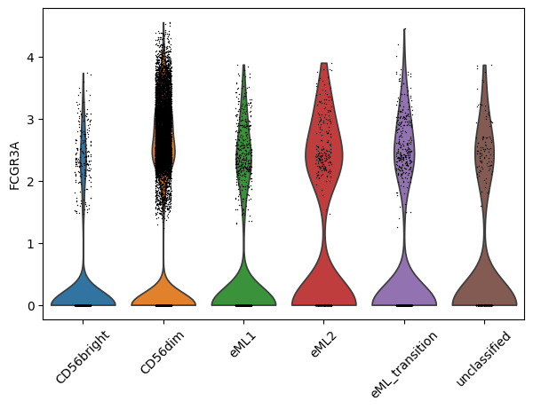
Visualize output data

Violin plot of selected gene in NK_type categories:

sc.pl.violin(adata_PBMC, ["FCGR3A"], groupby="NK_type", rotation= 45)

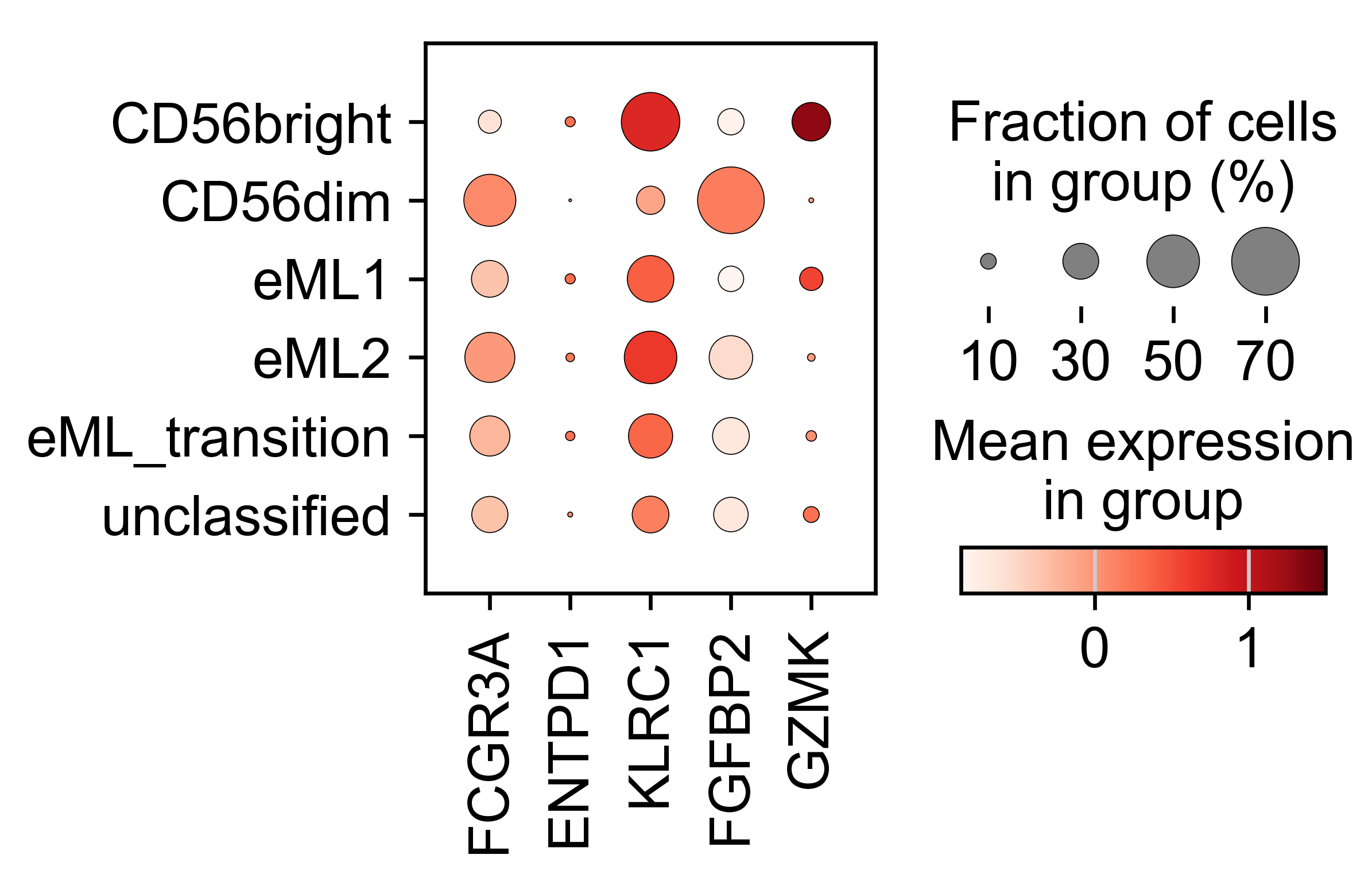
Dotplot of selected genes in NK_type categories:

genes= ["FCGR3A", "ENTPD1", "KLRC1", "FGFBP2", "GZMK"]

# Subset the adata object to include only the valid genes
adata_valid = adata_PBMC[:, genes]

# Scale the expression data for the valid genes
sc.pp.scale(adata_valid, zero_center=True, max_value=None)

# Generate a dot plot for the 'NK_type' column
sc.pl.dotplot(adata_valid, var_names=valid_genes, groupby='NK_type', vmax=1.5, use_raw=False, cmap='Reds')

Visualize ouput data more with Scanpy Documentation.

Note:

If you have preprocessed data already, you can initiate with defining command line arguments, loading reference model which is later followed by training the model with it’s next steps in interactive session.